Tutorial for Spline¶

Background information about B-spline at Wikipedia.

Splines from fit points¶

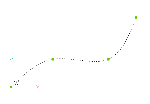
Splines can be defined by fit points only, this means the curve passes all given fit points. AutoCAD and BricsCAD generates required control points and knot values by itself, if only fit points are present.

Create a simple spline:

doc = ezdxf.new("R2000")

fit_points = [(0, 0, 0), (750, 500, 0), (1750, 500, 0), (2250, 1250, 0)]
msp = doc.modelspace()
spline = msp.add_spline(fit_points)

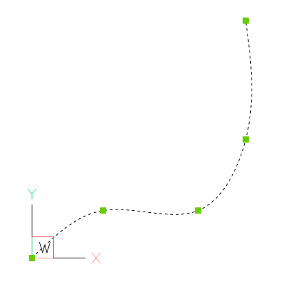
Append a fit point to a spline:

# fit_points, control_points, knots and weights are list-like containers:
spline.fit_points.append((2250, 2500, 0))

You can set additional control points, but if they do not fit the auto-generated AutoCAD values, they will be ignored and don’t mess around with knot values.

doc = ezdxf.readfile("AutoCAD_generated.dxf")

msp = doc.modelspace()
spline = msp.query("SPLINE").first

# fit_points, control_points, knots and weights are list-like objects:
spline.fit_points.append((2250, 2500, 0))

As far as I have tested, this approach works without complaints from AutoCAD, but for the case of problems remove invalid data from the SPLINE entity:

# current control points do not match spline defined by fit points
spline.control_points = []

# count of knots is not correct:
# count of knots = count of control points + degree + 1
spline.knots = []

# same for weights, count of weights == count of control points
spline.weights = []

Splines by control points¶

Creating splines from fit points is the easiest way, but this method is also the least accurate, because a spline is defined by control points and knot values, which are generated for the case of a definition by fit points, and the worst fact is that for every given set of fit points exist an infinite number of possible splines as solution.

To ensure the same spline geometry for all CAD applications, the spline has to be defined by control points. The method add_spline_control_frame() adds a spline passing the given fit points by calculating the control points by the Global Curve Interpolation algorithm. There is also a low level function ezdxf.math.global_bspline_interpolation() which calculates the control points from fit points.

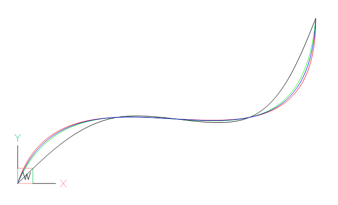
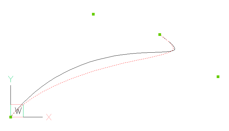
msp.add_spline_control_frame(fit_points, method='uniform', dxfattribs={'color': 1})
msp.add_spline_control_frame(fit_points, method='chord', dxfattribs={'color': 3})
msp.add_spline_control_frame(fit_points, method='centripetal', dxfattribs={'color': 5})

black curve: AutoCAD/BricsCAD spline generated from fit points
red curve: spline curve interpolation, “uniform” method
green curve: spline curve interpolation, “chord” method
blue curve: spline curve interpolation, “centripetal” method

Since ezdxf v1.1 the method add_cad_spline_control_frame() calculates the same control points from fit points as AutoCAD and BricsCAD.

Open Spline¶

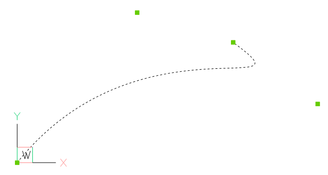
Add and open (clamped) spline defined by control points with the method add_open_spline(). If no knot values are given, an open uniform knot vector will be generated. A clamped B-spline starts at the first control point and ends at the last control point.

control_points = [(0, 0, 0), (1250, 1560, 0), (3130, 610, 0), (2250, 1250, 0)]
msp.add_open_spline(control_points)

Rational Spline¶

Rational B-splines have a weight for every control point, which can raise or lower the influence of the control point, default weight = 1, to lower the influence set a weight < 1 to raise the influence set a weight > 1. The count of weights has to be always equal to the count of control points.

Example to raise the influence of the first control point:

msp.add_rational_spline(control_points, weights=[3, 1, 1, 1])

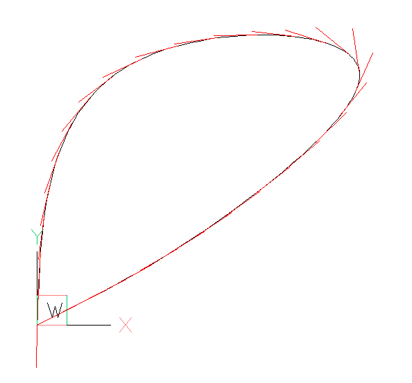
Spline Tangents¶

The tangents of a spline are the directions of the first derivative of the curve:

# additional required imports:
from ezdxf.math import Vec3, estimate_tangents
import numpy as np

# snip -x-x-x-

fit_points = Vec3.list(
    [
        (0, 0, 0),
        (1000, 600, 0),
        (1500, 1200, 0),
        (500, 1250, 0),
        (0, 0, 0),
    ]
)
spline = msp.add_spline(fit_points)

# draw the curve tangents as red lines:
ct = spline.construction_tool()
for t in np.linspace(0, ct.max_t, 30):
    point, derivative = ct.derivative(t, 1)
    msp.add_line(point, point + derivative.normalize(200), dxfattribs={"color": 1})

To get a smooth closed curve the start- and end tangents have to be set manually when the control points are calculated and they have to point in the same direction:

t0= Vec3(1, -1, 0)  # the length (magnitude) of the tangent is not relevant!
spline = msp.add_cad_spline_control_frame(fit_points, tangents=[t0, t0])

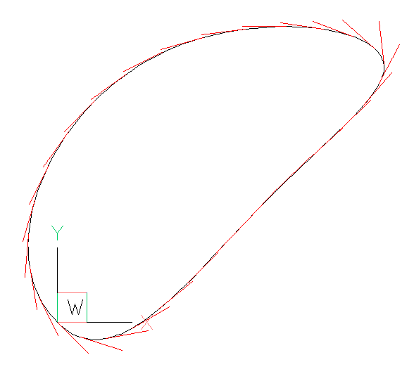
To avoid guess work the function ezdxf.math.estimate_tangents() can be used to estimate the start- and end tangents of the curve:

tangents = estimate_tangents(fit_points)
# linear interpolation of the first and the last tangent:
t0 = tangents[0].lerp(tangents[-1], 0.5)
msp.add_cad_spline_control_frame(fit_points, tangents=[t0, t0])

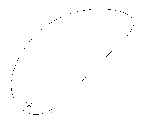
It is also possible to add the SPLINE by fit-points and setting the tangents as DXF attributes:

spline = msp.add_spline(fit_points)
spline.dxf.flags = spline.PERIODIC | spline.CLOSED
spline.dxf.start_tangent = t0
spline.dxf.end_tangent = t0

Spline properties¶

Check if spline is a closed curve or close/open spline, for a closed spline the last point is connected to the first point:

if spline.closed:
    # this spline is closed
    pass

# close spline
spline.closed = True

# open spline
spline.closed = False

Set start- and end tangent for splines defined by fit points:

spline.dxf.start_tangent = (0, 1, 0)
spline.dxf.end_tangent = (0, 1, 0)

Get data count as stored in DXF attributes:

count = spline.dxf.n_fit_points
count = spline.dxf.n_control_points
count = spline.dxf.n_knots

Get data count from existing data:

count = spline.fit_point_count
count = spline.control_point_count
count = spline.knot_count